St. Edward Road Proposal
FE 346:
Russ Foisy
Eric Forner
Matthew
Ghiorse
Bret Macaleer
Jeff Wale
March 12, 2001
St. Edward State park, Kenmore,
Washington
Table of Contents
Objectives (Matthew, Bret, and Jeff)
Site Description (Matthew)
Culvert Design (Nathan, Jeff)
Cross Drainage Design (Eric, Bret)
Curve Widening (Russ, Matthew, and
Eric)
Haul-time (Jeff, Matthew)
Ballast Design (Nathan Russ)
Clearing and Grubbing (Matthew)
Road Design (Bret)
Criterion
RoadEng
Costing
(Eric)
Objectives
Our main objective for this project
was to plot, traverse, stake out and cost a logging road in St Edwards State
Park. The primary function of this road is to transport harvested timber from
the landing site to a mainline.
Site Description
Our road site is located in
St.Edwards State Park, in Kenmore, Washington. It lies within sections 32 and
33,T.26n,R4E, and sections 4 and 5, T.25N,R.4E, W.M. Each member of the crew
team shared all responsibilities. The crewmembers were Nathan Werner, Russ
Foisy, Jeff Wale, Matthew Ghiorse, Eric Forner, and Bret Macacleer.
Culvert Design
Intro/Background
This crossing is being
installed because it is necessary to cross the creek in order to complete the
road decided in our FE 346 class. Due to
the fact that there are questions as to whether or not the creek could support
fish, the decision was made that the final design must allow for fish passage.
Culvert Design
Process Used in Design of
Culvert
The following, is the process and methods used in
determining an adequate culvert design. This process should be followed each
time a culvert design is undertaken, in order to account for all of the key
parameters.
Establish Givens/Assumptions
Side slope
ratios
Slope ratios for the culvert design have a direct
impact on the length of the culvert. For this reason, we used three different
slope lengths in order to aid us in deciding which would offer the most
advantageous results. There are no set slope ratios, but according to our specifications
we used 2:1 on either side of the curve over the stream. The steeper the slope the shorter the
culvert. The limiting factor here is that as the slope increases, cost
increases in order to minimize erosion. Although the 2:1 will erode the least with
minimal armament, the length of culvert is considerably longer. On the other
hand, if a 1:2 ratio is used, the culvert is much shorter, but the cost to
armor the slopes increases due to the need of retaining walls or rock gabions.
Assumed road width
The width of the road was assumed to be 26.2 feet
including the curve widening, in order to accommodate our design vehicle. The point of the crossing occurs at a curve
so that a 80 ft. radius was used in coming up with these specifications from
the info on curve widening taken from the 2.2 links, Forest Service Handbook
7709.56. The width of the road will also
act as a limitation on the length of the culvert, but cannot be varied.
Assumed height
of fill above culvert
The value of 14.5 feet from the flow line was also
taken into account to figure the total length of the culvert. We had to figure the added length do to the
2:1 ratio which added 58 feet to our culvert length.
Calculations
Stream
gradient
The stream gradient was estimated from the data
points and an estimated topographic map produced from Road Eng. The rise and run were measured in the section
of the creek where the culvert will be placed. The rise and run were then
divided to calculate a percent slope of 4%.
Length of
culvert
The total length of the culvert was figured through
means of the road and the side slope ratio and the total came out to equal 84.2
feet.
Discharge
values
The discharge values were calculated using the DNR
forest practices method. The Q
(discharge) values must be computed for the 100-year event for maximum passage,
and the 2-year event for the minimum flow and fish passage needs.
Equations:

Culvert
Dimensions
The dimensions of the culvert were calculated by
using the hydraulic charts for the selection of highway culverts prepared by
the U.S. Department of Commerce. The
arch culvert dimensions were 58inches by 36 inches.
Depth of water
in pipe
The depth of water in the pipe was calculated from
the dimensions of the culvert and the flow rate of a 2-year storm.
Velocity of
water in pipe
The velocity of the water in the culvert was
calculated using the equation Mannings Equation and then solving for V. From this we found that our velocity was 7.31
ft/sec which was found assuming the culvert was rectangular for the area that
the water reached. This value was not
appropriate for the fish to swim in because the velocity was to great. Therefore, we then assumed that we would put
in some boulders to slow the stream flow and got a knew value of n that equaled
.088 found in Environmental Hydrology book on page 223 table 7.5. From this assumption we then found a knew
velocity of 3.16ft/s which did meet the requirements of the fish to move up the
stream.

Hydraulic Drop
Since the culvert will be layed in at the same grade
as the stream bed, there will be no hydraulic drop.
Fish passage
Species
Although there are many possible fish species that
might use Miner Creek, the design fish is the trout that is < 6 inches.
Fish characteristics
The culvert is designed for a trout that is < 6
inches. This is because this fish is the limiting factor; all of the other
species can handle greater velocities and have similar needs in terms of depth.
This criterion was verified with Ken Bates of the Washington State Fish and
Wildlife Department.
Maximum
allowable flow velocities and depth requirements
|
Criteria: >6-inch adult trout |
Adult Pink, Steelhead |
Adult Chum Salmon |
Adult Chinook, Coho,
Sockeye |
|
Culvert Length (ft): |
Max. Velocity (ft/s) |
Max. Velocity (ft/s) |
Max. Velocity (ft/s) |
|
10-60 |
4.0 |
5.0 |
6.0 |
|
60-100 |
4.0 |
4.0 |
5.0 |
|
100-200 |
3.0 |
3.0 |
4.0 |
|
> 200 |
2.0 |
2.0 |
3.0 |
|
|
|
|
|
|
Flow Depth Minimum (ft): |
0.8 |
0.8 |
1.0 |
|
Hydraulic Drop Maximum
(ft): |
0.8 |
0.8 |
1.0 |
Table from WAC
220-110-070
It is clear that the maximum allowable velocity for
the flow in the culvert cannot be greater than 4 ft per second, for culverts
between 1 and 200 feet in length. This specific aspect will not allow this
design to pass fish because the culvert velocity is 13.8 ft per second.
Cost = 15.48*84.2+29.98*84.2
= 3827.73
Cross Drainage Design
Using
the following graph for determining cross drain spacing we came up with
3136.64kg per year being a tolerable sediment load and therefore considering
our average slope to be about 8% we used the cross-drain spacing of 60 m.
|
Climate
station: |
Sappho,
WA |
|
Buffer length: |
200
m |
|
Soil type: |
graveled
loam |
|
Buffer gradient: |
60
% |
|
|
|
|
Road width: |
4
m |
Average
annual sediment yield (kg)
|
Road |
Cross drain spacing |
||||
|
10 m |
30 m |
60 m |
120 m |
240 m |
|
|
2 % |
512.64 |
969.12 |
1840.36 |
4097.84 |
10334.48 |
|
4 % |
547.88 |
1136.80 |
2328.20 |
5722.04 |
15737.64 |
|
8 % |
608.56 |
1416.36 |
3136.64 |
8260.56 |
24350.16 |
|
16 % |
702.16 |
1848.84 |
4402.52 |
12162.32 |
36779.84 |
Sappho 8 E Snider Ranger Station,
WA USA -- August 1999
USFS Rocky Mountain Research Station, Moscow
Then
using RoadEng we put 18” diameter culverts of various lengths at skew angle of
60 degrees and sloped at –4%. A total of
10 cross-drains were put in. The arch
for the stream was already put in, but we added it in to our cost calculation
The
Total cost for the cross-drains was $4678.65
|
Culvert length |
install cost |
Furnish cost |
subtotal |
|
|
30 |
8.44 |
8.21 |
499.5 |
|
|
22 |
8.44 |
8.21 |
366.3 |
|
|
29.5 |
8.44 |
8.21 |
491.17 |
|
|
31.25 |
8.44 |
8.21 |
520.31 |
|
|
23.5 |
8.44 |
8.21 |
391.27 |
|
|
32 |
8.44 |
8.21 |
532.8 |
|
|
20 |
8.44 |
8.21 |
333 |
|
|
39 |
8.44 |
8.21 |
649.35 |
|
|
33 |
8.44 |
8.21 |
549.45 |
|
|
20.75 |
8.44 |
8.21 |
345.48 |
|
|
total |
|
|
4678.65 |
|
|
Stream arch |
|
|
3827.73 |
|
Grand
total 8506.35
Curve Widening
One
of the key elements to designing a low volume road is deciding on what sorts of
vehicles are going to be traveling on the road and how often. There are two main types of vehicles used in
the road design. There is the design vehicle, which will use the road the most
of any vehicle and should be able to travel the length of the road unassisted.
There are the critical vehicles, which will use the road only a few times and
may need help through trouble spots, such as filling in the ditch line to make
a tight curve.
In
our road design we have decided that the design vehicle is a standard log
truck. Our critical vehicles are a self-propelled yarder and a low boy
configuration large enough to bring in a loader.*
After
the road has been traversed and plotted, it is essential to ensure that all of
the vehicles that need to use the road at least once are able to get around the
curves. This adjustment is called curve widening.
A
standard road has a travel width of twelve feet. Due to the length and size of
the vehicles, all of them have there own specific traveling width especially
around curves. Therefore our first step is to calculate the curve widening
needed for each vehicle around each curve. This is done by establishing the
radius of the curve, knowing the central angle of the curve and using the specs
for the vehicle to attain a length.
Standard
log truck:
L = ![]()
L1 = wheel base
of truck
L2 = length of stinger
L3 = Bunk to
bunk distance minus the length of stinger.
Low
boy configuration:
L = ![]()
L1 = wheelbase of
truck.
L2 = distance from the 5th
wheel to the middle of the rear duel wheels for the first trailer.
L3 = distance from the 5th
wheel to the middle of the rear duel wheels for the second trailer.
*
All of the specifications for these vehicles can be found in the attached
appendices.
From
Figure 1 we can see that L1 is 6m which is 19.685 ft. L2
is 2.6m or 8.531 ft. L3 is 10.5m – 2.6m or 7.9m which is 25.92ft.
Therefore
Calculating L for the log truck:
L = ![]()
L = 31.408 ft
Calculating L for the lowboy:
L = ![]()
L = 46.25 ft
Our
first switch back has a radius of 60 ft and a central angle of 180°. Using the curve widening formula found in
Forest Service Handbook (FSH) 7709.56, 4.2 – 4.2txt fill.
CW = 
Again
for the log truck we found
CW = 
CW = 7.4 ft
These
calculations were done for each curve for the log truck and the lowboy.
We
found that there are no equation to find the curve widening for our yarder, so
we had the use a drafting simulator, which allowed us to represent a scale
model of our yarder and our curve. We then traced our yarder along the curve
and determined our curve widening for our scale representation.
Here
are our results:
|
Curve |
CW
for Log Truck (ft) |
CW
for Low Boy (ft) |
CW
for Yarder (ft) |
|
R
= 60 ft D
= 180° |
20.8 |
39.6 |
29 |
|
R
= 70 ft D
= 180° |
19.4 |
26.1 |
28 |
|
R
= 75 ft D
= 162.4° |
19.4 |
26.1 |
27 |
|
R
= 80 ft D
= 83.6° |
19.1 |
21.6 |
24 |
|
R
= 120 ft D
= 26.98° |
15.07 |
14.3 |
22 |
Table 1. Curve Widening
Results
As
we discussed our results we concluded that the low boy took precedence over all
the other vehicles in all of curves except, our 120 ft radius curve, due to the
large amount of curve widening needed.
Taper
is needed to integrate our curve onto our road:
The values we used for each curve are as
follows and were determined by Table 2:
|
Curve
Radius (ft): |
Taper
Length (ft): |
|
60 |
60 |
|
80 |
50 |
|
75 |
50 |
|
70 |
50 |
|
120 |
30 |
Table 2: Taper lengths
Curve
widening tapers should be straight lines before the point of curvature (PC) and
after the point of tangency (PT) for the following lengths:
Radius
(R)(feet) Taper Length (feet)
Less
than 70 60
70-85 50
86-100 40
Greater than 100 30
Haul Time
The
over all calculations found for haultime were calculated using the computer
program Otto Truck Simulator. In order
to use this program the following operations need to be performed.
First
the following road information must be obtained and recorded in a tab delimited
file from the road eng. map: Distance from beginning of the road to a point at
the beginning of a curve for each curve in the road in meters (straight lines
are considered a curve with infinite radius), the slope at the beginning of
each curve in decimal format, the radius of each curve (straight lines are
reported as a 99999 meter curve), the legal speed limit of the road section in
km/hr, and the surface type on a 1 to 10 rating (ratings can be found in the
Otto Truck Simulator instruction manual).
Next
the Otto program needs to be opened in DOS and the following information must
be inputted into the system: First truck specs are needed including engine and
transmission desired (these can be selected from the choices given from the
program), and the road file from the previous step must be imported as a ASCII
file. The program will then ask for gear
ratios and truck weights (weights will be needed for a loaded and unloaded
truck).
Once
all this information is inputted the Otto program will try to calculate
haultime. If the transmission does not
match the engine type or other problems the program will then inform you and adjustments
can be made.
The
following data will be supplied by Otto: Distance to the next station, time of
travel to the next station, speed between stations, power used, fuel
consumption rates, fuel consumed, rpm's, and the gear used between stations.
Ballast Design
Our
area had 1,000,000 Board feet and was logged in four years. The things taken into account were trips of
vehicles especially loaded log trucks, empty log trucks, yarders and
maintenance vehicles.
The
Log truck has a capacity of 5,000 board feet and will make approximately 200
trips over 4 years. The empty log truck
will make the same amount of trips and the maintenance vehicle will make
approximately 230 trips. Also, the
yarder will make 10 trips.
We
used a Surface Thickness Program from the Forest Service Department of
Agriculture. Table 1, Table 2, and Table
3 show the steps followed.
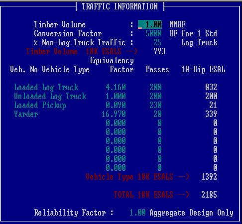
Table
1. Traffic Information. This information was given to us based on
usage of the road.
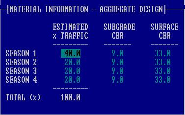
Table
2. Material Information. This contains the information on the soil
types at the site. The site had gravel
loam and from a compaction chart in Earth and Aggregate Surfacing Design
Guide for Low Volume Roads from the Forest Service (pg. 32), we figured
that it had a CBR of 9. Our Surface grade
is to be high end, so we are using a well graded crushed rock, which has a CBR
of 33.
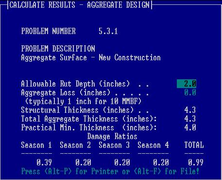
Table
3. Results. This takes the input from the first two
tables returns calculations here.
From
Table 3, we see that there should be a minimum grade thickness of 4.3
inches. We take this value to be 5
inches and then multiply by 2. The
maximum thickness of a particle is 5 inches and so the ballast thickness should
be twice that size giving us a thickness of 10 inches.
The
total volume of the ballast is 1172.2 cy3 (bases on RoadEng). The ballast cost is $7.50 per yd3. The cost to install it is $4.50 per yd3. This is a total of $12.00 per yd3.
The
total cost of the ballast installed is $14,066.40.
Clearing and Grubbing
Clearing is the process of removing (felling) timber from the right of way
Grubbing is the process of removing stumps/rootwads from the construction area
typically
a common cost value for clearing & grubbing is $ 600.-/acre
We
calculated the total surface area of our road, taking into consideration all
the curve widening, and calculated our road is 40,390 sq. ft. This converts to
.927 acres. From above we know that it costs $ 600 per acre to clear and grub.
This gives us a total of
Clearing and Grubbing:
$556.34.
Road Design
Criterion
The
Technical Use of the Criterion Survey Laser
The
laser while developed for timber cruising is very useful as a road survey
instrument. It can accurately measure horizontal distance, slope distance,
azimuth and percent slope. The laser also gives one the power to store the data
in the field; this reduces the human error involved in the relay of data from
the instrument operator to the note-taker. This also becomes rather enjoyable
when working in wet weather. This however does not mean that the laser is waterproof,
it can withstand a rainstorm, but do not throw it in a stream.
Equipment Needed To Operate
1. Criterion Laser
2. Reflector
3. Batteries and Cables
4. Foliage Filter
5. Shoulder Stock and Strap
6. A Competent Operator
Navigating the Criterion
Interface
The
criterion data display is limited to only two lines of text. Designated buttons on the control panel
controls the display. Up, down, and side
to side arrows allow the user to scroll through the text. Options are in folder type arrangement with
folders opening up to reveal other folders until a final selection is
made. Once an option is highlighted it
can be selected by pressing the 'Enter' button.
The 'Exit' button will take the user back to the previous folder.
Procedure for Criterion 400
(starting a unit survey)
1) Push the 'POWER'
button. (The word TREE should be displayed)
2) Use the up and down arrows to
Navigate; Go until you find SURVEY
and hit 'ENTER'
3) Then scroll until you find UNIT SURVEY and hit 'ENTER'. This will be displayed:
|
*SVY* |
(#) |
|
UNIT |
(#) |
(The asterisks can be moved
with the up and down arrows. Choose the numbers that you want to start with
preferably 1 and 1. Each unit number
will correspond to a saved unit survey.
The unit # cannot be zero or repeat something that has been saved)
4) When done use the down key to get to the next menu. (If
this does not work push enter then
the down arrow)
5) Scroll down to the screen:
|
*FROM* |
1 |
|
TO |
2 |
(This screen indicates the
point you are shooting from and the point you are shooting to. Each shot taken will create a point at the
target of the shot. Your first shot must
be a fore shot and will be from point 1 to point 2. Each side shot also counts as a point.)
6) Then down arrow until you see:
|
*FS* BS |
SIDE |
|
USER |
|
7) Make sure that the asterisks
are on the FS selection for the
initial shot. If it is not use the left
arrow button to select it.
8) Push the down arrow to see
the following screen:
|
HD: |
FT |
|
AZ: |
DEG |
(A shot can only be made
when the display shows this screen.
Otherwise the criterion will not take a reading.)
9) Take a reading at eye level
to approximately the same height on your partner or tree. Take first reading to the Left. To do this,
push the button on the hand trigger and hold it in. The longer you hold the
more accurate reading but shorter the battery life will become.
10) You have completed your shot
and can scroll up or down to view the data that has been collected.
11) Scroll until you find:
|
FS BS |
*SIDE* |
|
USER |
|
12) Push the orange
"SIDE" key (which is also the #5 key)
13) Scroll down to:
|
HD: |
FT |
|
AZ: |
DEG |
14) Take a side shot.
15) Push the orange 'SIDE' key
again to take another side shot.
16) Repeat this process to get
as many side shots as you like.
17) Scroll up to:
|
FS BS |
*SIDE* |
|
USER |
|
18) Press the 'INLINE' key. The asterisks should now be on the BS selection.
19) Place the criterion over the
next point in your road. (this should be
where your fore sight target was placed)
20) Use the down arrow once to:
|
HD: |
FT |
|
AZ: |
DEG |
21) Take your back shot.
22) Now you are ready to repeat
the process. Make sure that you follow
your back shot with a fore shot before shooting side shots.
23) Go back to step 1
Note taking for the Criterion
· Set up your rite in rain notebook like the one shown in Figure 1 below.
·
Begin recording your data at the bottom of the left-hand page and work
your way up the page. *
·
Your first shot should always be a foresight.
·
After every Foresight, at least two sides shots should be
observed and recorded for data to calculate cross sectional areas. These shot
should be taken perpendicular to the road, and one taken in each the downhill
and uphill directions. These are the bare minimum required. You should take
more shots further away, or at different angles from the point. The flatter the
terrain, usually more side shots can be taken to acquire an efficient map of
the terrain. All of this information is recorded on the right-hand side of the
page. The essential information needed when taking side shots is distance, which gets recorded on the
bottom and slope grade, which gets
recorded on the top.
·
You then will proceed to the next point and there you take a backsight
to the previous point and then another foresight to the next point. Then repeat
above.
·
Be sure to leave ample space on the left-hand side of the notebook
between foresights and backsights. This allows enough room to on the right hand
side of the notebook to record your sideshots and any other pertinent notes
that need to be addressed.
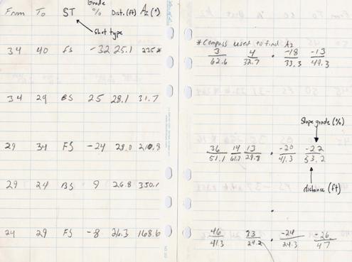
Figure 1: example of field notes
RoadEng
Data Transfer
The
road data was transferred from an Excel file into RoadEng using the import
feature. The data came into excel in a
comma delaminated form. The FE Handbook
describes the following steps for creating a terrain model in RoadEng:
Transfer .pol files to RoadEng.
- Open Softree 98 then
select the Terrain mode.
- In the Terrain mode,
go to File and select Import
- From the small window,
select UNIT SURVEY and click on
Options.
- From the Options window, select the
following features and then click on OK.
- Softree will take you
back to the Import window, click OK.
- From the Unit Survey
window, find the .pol file that you saved and click on OK.
- Softree now creates
the plan view of your road.
If the plan view does not
resemble the layout of the site that was observed or the plan view seems to be
incomplete, the data obtained from the field needs to be rechecked.
- To calculate the
Terrain model, go to Edit
then select Calculate
Terrain Model and choose the following features and click on OK. This option from Softree will
calculate the contour lines on the Plan view of your road.
- A plan view the
contour lines is created from the Terrain Calculation option. You can adjust the contour intervals by
going back to Step 8 and changing the contour intervals. After the
contour lines are added to your plan view, save the file as a .ter file.
Terrain Module
In the Terrain module, errors in the data were
fixed. There were a few areas where
obvious mistakes had been made in recording the data. These areas were adjusted to the location
that we predicted them. During data
collection a connecting line was run from the end of the road to a control
point on the road. This line was removed
in the Terrain module. The data was transferred from the Terrain module to the
Location module. The following steps
were performed as found in the FE Handbook.
Transferring data to the Location mode.
- From the Edit menu, select Select Feature(s) and click on All.
- From the File menu, select Export Feature…and click on Ok.
- A Traverse Document
Export file window will be shown which allows you to save your file with
a .db1 extension.
- A warning window may
be shown notifying that the side slope extends outside of the Terrain
Model. Select OK.
- From Module, select to Location screen. From the File
menu or the open folder icon, select the .db1 file that you have created.
The Survey/Map screen opens the file in a similar format as the Field
notebook.
- To view the Profile
and cross sections of your road, select from the Module menu To Location Design. Select New
from the File menu or
click on the New icon
and a Select P-line traverse window will be shown. Find you .db1 file and click OK.
Location
Module
Windows
The majority of the design work
was performed within the Location module.
The four windows that were created were the plan, section, profile, and
data windows.
Profile window
In this window the gradeline
was adjusted according to the desired slope.
Here adjustments can be made to the vertical location of the road. Vertical curves were created to smooth the
transition between grades. A mass haul
subwindow was created here. This was
adjusted by creating mass haul waste locations.
Plan window
This window shows and
overhead view of the road. Here
adjustments can be made to the horizontal location of the road. Horizontal curves were created to smooth the
transition between straight-aways. This
window also shows the road width.
Section window
This window shows a cross
section view of the road prism. No
adjustments are made here in this view.
It is only for reference.
Data window
This window shows all data
sets in tabular format. The columns can
be chosen from the view menu.
Templates
Road prism templates were
created for each curve, straightaway, and taper. These templates were assigned to the proper
road locations. Here the road width,
ballast height, and side slopes were specified.
Culverts
Culverts were inserted into RoadEng
using the Edit Culvert function in
the Edit menu. The depth and length were adjusted here to
fit each location.
Costing
|
Clearing and Grubbing |
|
$556.34 |
|
Culverts and Stream Arch |
total = $8506.35 |
|
|
|
Culverts |
$4678.65 |
|
|
Stream Arch |
$3827.73 |
|
Ballast Costs |
|
$14,066.40 |
|
Haul time costs |
|
$811.37 |
|
Excavation |
|
$31,052.00 |
|
Grand Total |
|
$54,992.50 |
Appendix